How to Edit Data in Microsoft Excel

Co-authored by wikiHow Staff

Last Updated: December 18, 2022 References

If you're not very familiar with Microsoft Excel, it might seem an intimidating program to use. Fortunately, it's easy to get started. You can type in data, copy and paste it from other documents, and format it with just a few clicks. With a little practice, you'll be able to quickly enter, edit and manage data in Microsoft Excel.

Part 1

Part 1 of 3:

Entering and Selecting Data

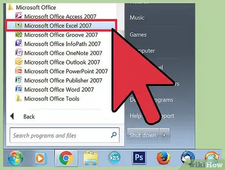
1
Launch Microsoft Excel. You can locate Excel by clicking the "Start" menu, selecting "All Programs," selecting "Microsoft Office" and then choosing "Microsoft Excel." Excel comes with the Microsoft Office suite of products generally packaged with Windows computers and notebooks.
- Mac users who have purchased Excel for Mac will find the program located in their Dock or among by opening "Finder" and then selecting "Applications."
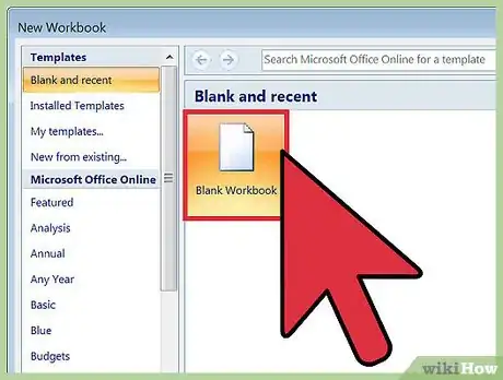
2
Open a spreadsheet. A blank "workbook" may automatically appear upon opening Excel. Otherwise, you'll see a "Template Gallery" from which you can either select a new blank workbook or a specially formatted template.
- You may always open a new spreadsheet while working on another workbook in Excel. Simply click on "File" from the menu bar and select the "New Workbook" option.
Advertisement
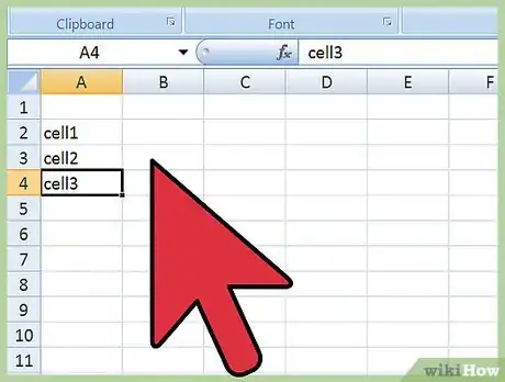
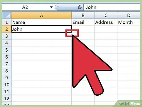
3
Enter data into desired cells. You may type numbers, words, equations, formulas or functions in any cell after selecting and clicking on it. ^{[1]
X
Research source}
- When finished with a given cell, press ↵ Enter or Tab ↹ to automatically move to the next cell horizontally.
- You may also create a new line within a cell on which to add more text. Simply enter a "Line Break" by pressing Alt+↵ Enter.
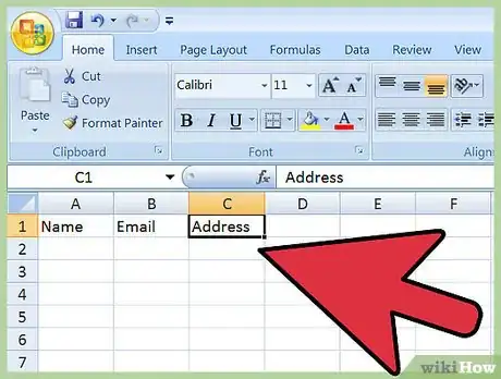
4
Create headings for your columns. Enter text into Row 1 to create column headings for your data. For instance, enter "Name" into cell A1 and “Date” into cell B1 and allow these to serve as your column headers for tracking name and date information.
5
Create a sequenced data series. Excel is able to learn patterns underlying your data and then fill in data based on those pattern to save you time and energy. Begin by establishing a pattern in consecutive cells (e.g. typing "January" in one cell and "February" in the next). Then select the populated cells and click and drag the bottom right corner of your selected rectangle to expand the pattern into new cells. Excel will automatically recognize your established pattern and fill in subsequent cells with "March", "April" and so on.
- Excel can recognize many common patterns such as days of the week, evenly-spaced dates, consecutive numbers and many others.
6
Select a range of cells. To select a range of cells with via your mouse (in order to format or edit larger quantities of data), simply click the beginning or end of a data range and drag your cursor in your desired direction to highlight the appropriate text. There are also a number of helpful keyboard shortcuts enumerated below.^{[2]
X
Research source}
- Pressing Ctrl and the spacebar extends a selection throughout the column where the original cell is located.
- Pressing ⇧ Shift and the spacebar extends a selection throughout the row where the original cell is located.
- Pressing Ctrl+⇧ Shift and the spacebar or Ctrl+A will select the entire worksheet.
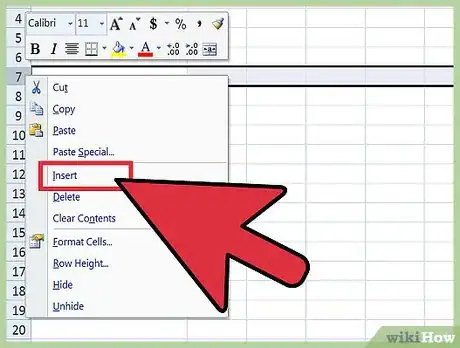
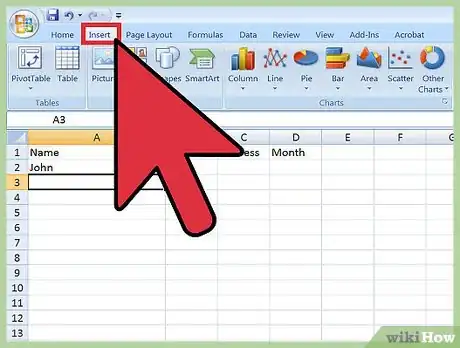
7
Insert row(s). Begin by clicking a row number (this will select the entire row). Select the row that you'd like your new row to go above. Right-click (Control+click on Mac) and select "Insert" from the menu that appears.^{[3]
X
Research source}
- This function is also available from the "Home" tab by selecting "Insert" from the "Cells" then "Insert Sheet Rows."
- Inserting multiple rows requires you to select multiple rows above the location in which you wish to place new rows. Simply select the same number of rows that you want inserted below.
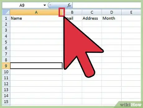
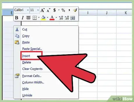
8
Insert columns(s). Begin by clicking a column letter (this will select the entire column). Select the column that you'd like your new column to go to the left of. Right-click (Control+click on Mac) and select "Insert" from the menu that appears.
- This function is also available from the "Home" tab by selecting "Insert" from the "Cells" then "Insert Sheet Rows."
- Inserting multiple columns requires you to select multiple columns to the right of the location in which you wish to place new columns. Simply select the same number of columns that you want inserted to the left.

Part 2

Part 2 of 3:

Editing Data

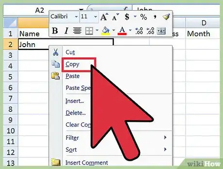
1
Copy one or more cells. After selecting the cell(s) you wish to copy, right-click and select "Copy" from the menu that appears. Alternately press Ctrl+C (or ⌘ Command+C for Mac users). This will add the selected data to your clipboard.
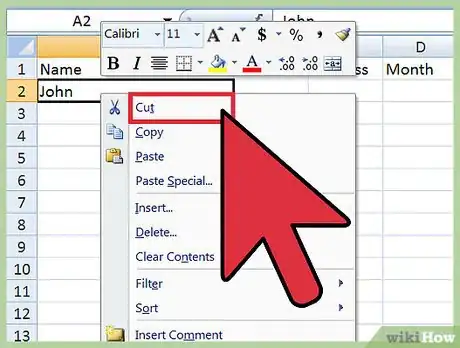
2
Cut one or more cells. After selecting the cell(s) you wish to cut, right-click and select "Cut" from the menu that appears. Alternately press Ctrl+X (or ⌘ Command+X for Mac users). This will add the selected data to your clipboard.
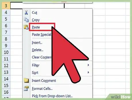
3
Paste one or more cells. After selecting the cell(s) in which you wish to paste your data, right-click and select "Paste" from the menu that appears. Alternately, press Ctrl (or ⌘ Command for Mac users). This will paste the contents of the copied or cut cell(s).
- If your cell contains a formula, "Paste" will paste the formula not calculated value of the formula. In order to "Paste" cell values, use "Paste Special"
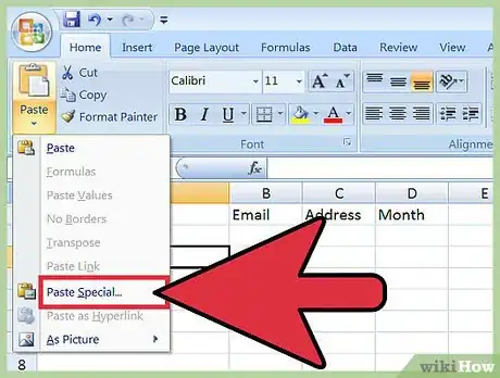
4
Paste cell values instead of formulas. Begin by selecting "Edit" from the "Home" tab and clicking "Paste Special." Select "Values" from the list of attributes to paste. ^{[4]
X
Research source}
- Depending on your version of Excel, other options in the "Paste Special" may include "Comments" (text comments which can be added to individual cells), "Formats" (all text formatting selections), or "All" to paste everything at once. ^{[5]
  X
  Research source}
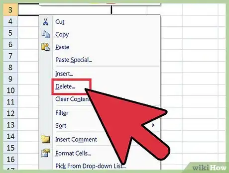
5
Delete cell content. Simply select the cell(s) in which you wish to delete text and press Del or right-click and select "Delete" from the menu that appears.
6
Move cells, rows or columns. Highlight your chosen cells and activate the "move pointer" (appearing as four directional arrows for Windows users or as a hand icon for Mac users). Drag to your preferred location to replace any existing data there with the cells you've decided to move^{[6]
X
Research source}
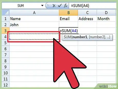
7
Use a formula. Excel uses "formulas" to make calculations within a cell and can reference other cells as part of that calculation. Click the cell in which you wish to enter the formula and then begin by typing "=". Now type a mathematical formula and click "Enter". Excel will display the results (not the formula itself).
- You can also learn more about How to Type Formulas in Microsoft Excel
8
Reference values from other cells. Formulas can reference other cells and their values. While typing a formula, simply click a single cell or a range of cells and Excel will automatically populate the cell's name (e.g., B2, D5) into your formula. Now your formula references that specific cell and will draw a value from it continuously. If the value in the referenced cell changes, the results of your formula will as well.
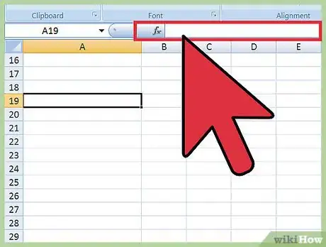
- You can also reference values from other worksheets. Begin by selecting the cell in which you wish to reference a value, type an "=' in the formula bar and then type your desired formula immediately after the "=." After typing the formula, simply click on the tab for the worksheet you wish to reference and then select the desired data range that you want entered into the formula.
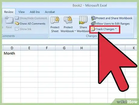
9
Track your changes. You can track changes by selecting "Tools" from the menu bar and then clicking "Track Changes." Finally, select "Highlight Changes."
- If this option is unavailable, you are in a Read-Only format. Under "Track Changes," check the option next to "Track changes while editing. This also shares your workbook." Once this option is selected, then you can make changes and view those changes by selecting this option again and checking the box next to "Highlight Changes."
10
Add comments. This can be a useful way to discuss edits made on an Excel spreadsheet. Begin by selecting the cell(s) on which you wish to comment. Then select "Insert" from the menu bar and click "Insert Comment" from the menu that appears. A text box will appear in your desired location and allow you to leave a comment.
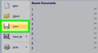
11
Save your changes. Select "File" from the menu bar and click "Save." Then select the "Save In" drop-down list button and choose your preferred folder. If you attempt to exit Excel before saving your most recent changes, a dialogue box will appear and ask if you wish to save your changes. You may either click "Save" or "Don't Save" depending on your preference.

Part 3

Part 3 of 3:

Formatting Data

1
View the "Format" ribbon. Be sure that the "Format" ribbon is visible so that you can easily and quickly access a variety of formatting options. Simply click the downward-pointing arrow at the right side of the "Format" ribbon to expand it. This will allow you to adjust font style and size while also making text italicized, bold or underlined. It also gives you shortcut access to several of the functions discussed in formatting steps outlined below. ^{[7]
X
Research source}
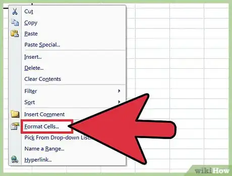
- A right-click on a cell or group of cells also brings up formatting options. After right-clicking the cell(s), select "Format Cells." This will provide you a number of options with respect to Number (style), Alignment, Font, Border, Patterns and Protection.
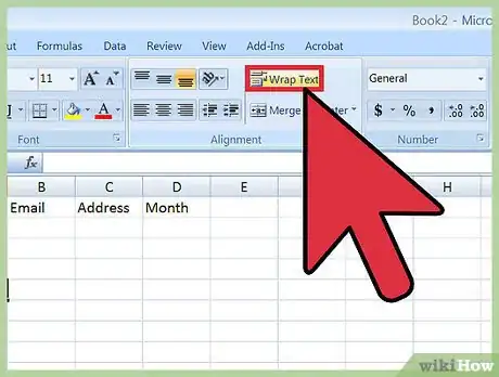
2
Wrap your text. This will cause text to wrap around and remain visible within a cell rather than trailing off and becoming obscured by the next cell. Begin by highlighting the cells you wish to adjust. Then, under the "Home" tab, look at the "Alignment" group of buttons and select the "Wrap Text" option.
- You can also adjust your text to fit cells so that columns and rows automatically adjust their width or height (respectively) in order to accommodate the content within a cell. Under the "Home" tab, look at the "Cells" group of buttons and click "Format." From the "Format" menu, select "Cell Size" and click either "AutoFit Column Width" or "AutoFit Row Height."
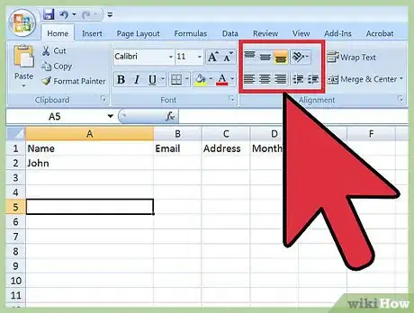
3
Align your text. This will cause your text to be justified on the left, right or center part of the cells. Begin by highlighting the cells you wish to adjust. Then, under the "Home" tab, select the appropriate alignment. You'll see three buttons with lines oriented so as to demonstrate the side of the cell(s) in which text will begin.
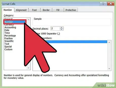
4
Change the numeric style of data. You'll find several basic numbering styles on the "Format" toolbar itself. Simply select the cell(s) you wish to format and then click the appropriate numeric style located on the toolbar. To access additional styles, right-click on the selected cell(s), click "Format Cells" and then select the "Number" tab. You'll see a variety of options listed under "Category."
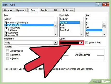
5
Change your text color. Select the cell(s) for which you wish to adjust the text color. Then, from the "Format" toolbar, click the downward pointing arrow next to "Font Color." This is the option that looks like a letter "A" with a colored line underneath it. Clicking the arrow with display a menu with a variety of color options.
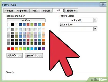
6
Change your background color. Select the cell(s) for which you wish to adjust background color. Then, from the "Format" toolbar, click the downward pointing arrow next to "Fill Color." This is the option that looks like a letter paint can with a colored line underneath it. Clicking the arrow with display a menu with a variety of color options.

Community Q&A

Question

I want to edit information in an Excel spread sheet, but I can't alter information in the cells.

Community Answer

Your Excel document may be in "Read Only" mode. After opening Excel, click the "Office Orb" at the upper, lefthand side of the screen and select "Open" to access your desired document. Then click that orb again and select "Save As." Then select the "Tools" button next to "Save" and click "General Options." Finally, uncheck the box located next to "Read-only," click "OK" and select "Save" for the changes to take effect.
Question

How do i change background colors?

Community Answer

First, select the cell(s) for which you wish to change the background color. Then, from the "Format" toolbar, click the downward pointing arrow next to "Fill Color." This is the option that looks like a letter paint can with a colored line underneath it. Clicking the arrow with display a menu with a variety of color options.
Question

How do I create a worksheet?

Community Answer

A blank "workbook" may automatically appear upon opening Excel. Otherwise, you'll see a "Template Gallery" from which you can either select a new blank workbook or a specially formatted template. You may always open a new spreadsheet while working on another workbook in Excel. Simply click on "File" from the menu bar and select the "New Workbook" option.