How to Add a Filter in Excel 2007

Last Updated: February 15, 2023

You can use filters in Microsoft Excel to show only the data that meets certain conditions. We'll show you how to set up an AutoFilter in Microsoft Excel 2007 to filter a column by date, color, or any other criteria.

Method 1

Method 1 of 2:

Applying Filters

1
Open the spreadsheet in which you want to filter data.
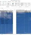
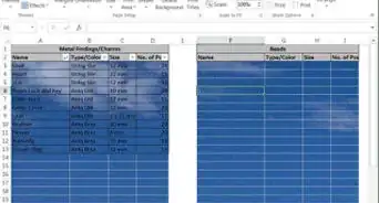
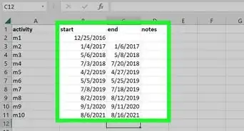
2
Prepare your data for an Excel 2007 AutoFilter. Excel can filter the data in all selected cells within a range, as long as there are no completely blank rows or columns within the selected range. Once a blank row or column is encountered, filtering stops. If the data in the range you wish to filter is separated by blank rows or columns, remove them before proceeding with the AutoFilter.
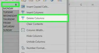
- Conversely, if there is data on the worksheet that you do not want to be part of the filtered data, separate that data using one or more blank rows or blank columns. If the data you don't want to filter is located beneath the data to be filtered, use at least one completely blank row to end filtering. If the data you don't want to filter is located to the right of data to be filtered, use a completely blank column.
- It is also good practice to have column headings within the range of data being filtered.
Advertisement
3
Click any cell within the range that you would like to filter.
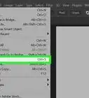
4
Click the "Data" tab of the Microsoft Excel ribbon.
5
Click "Filter" from the "Sort & Filter" group. Drop-down arrows will appear at the top of each column range. If the range of cells contains column headings, the drop-down arrows will appear in the headings.
6
Click the drop-down arrow of the column containing the desired criteria to be filtered. Do one of the following:
- To filter the data by criteria, click to clear the "(Select All)" check box. All other check boxes will be cleared. Click to select the check boxes of the criteria that you want to appear in the filtered list. Click "OK" to filter the range by the selected criteria.
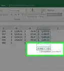
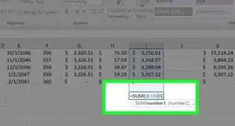
- To set up a number filter, click "Number Filters" and then click the desired comparison operator from the list that appears. The "Custom AutoFilter" dialog box appears. In the box to the right of the comparison operator selection, either select the desired number from the drop-down list box or type the desired value. To set up the number filter by more than one comparison operator, click either the "And" radio button to indicate that both criteria must be true, or click the "Or" radio button to indicate that at least 1 criterion must be true. Select the second comparison operator, and then select or type the desired value in the box to the right. Click "OK" to apply the number filter to the range.
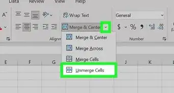
- To filter the data by color-coded criteria, click "Filter by Color." Click the desired color from the "Filter by Font Color" list that appears. The data is filtered by the selected font color.

Method 2

Method 2 of 2:

Removing Filters

1
Click the drop-down arrow of the range containing the filter and then click "Clear Filter from Column Heading," to remove filtering from one column.
2
Click the "Data" tab of the Microsoft Excel ribbon and then click "Clear" to clear filters from all columns.

Community Q&A

Question

How do I select a column in Excel?

Community Answer

Click the box with the sequence of letters that corresponds to the column you want to select. For example, if you wanted to select column D, click the box with "D" on it.
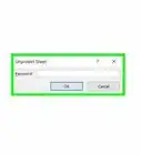
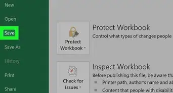
Question

How do I save my filters?

Community Answer

There is a save icon in Microsoft word that lets you save your files. It looks like a floppy disk. You can also press the control key and the letter 'S' at the same time to save your files. That is the keyboard shortcut for save.
Question

How many type of filters are there in MS Excel?

NurtureTech Academy

Community Answer

There are two types of filters available in MS Excel: filter and advance filter. Filters are just normal filters which are applied on the upper side of the sheet with a shortcut key (Ctrl+Shift+L). Advance filters are used when you want to apply more than one condition to the data, or you want to extract data on a different sheet.